Introduction
In ANALYZING GREENNESS THROUGH NDVI IN REDLINED AREAS IN PHILADELPHIA, PENNSYLVANIA the main focus was on applying the remote sensing skills developed through the course to be able to quantify and explore simple relationships between variables. Here I extend that previous work by applying statistical concepts learned in EDS 222 Statistics for Environmental Data Science.
HOCL ‘Redlining’
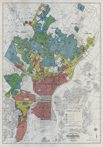
‘Redlining’ is the term used for the racist, nativist, and class privileged maps and its grading system created by the Home Owners Loan corporation (HOCL) under the New Deal federal stimulus program of 1935. These HOCL grades and maps were used by mortgage lenders for decades furthering racial segregation and a disparity in financial resources
A = Best
B = Still Desirable
C = Declining
D = Hazardous
Example of language used to describe region D: • “Undesirable negro section of very poor property”
• “Concentration of undesirables. Low class whites and negro”
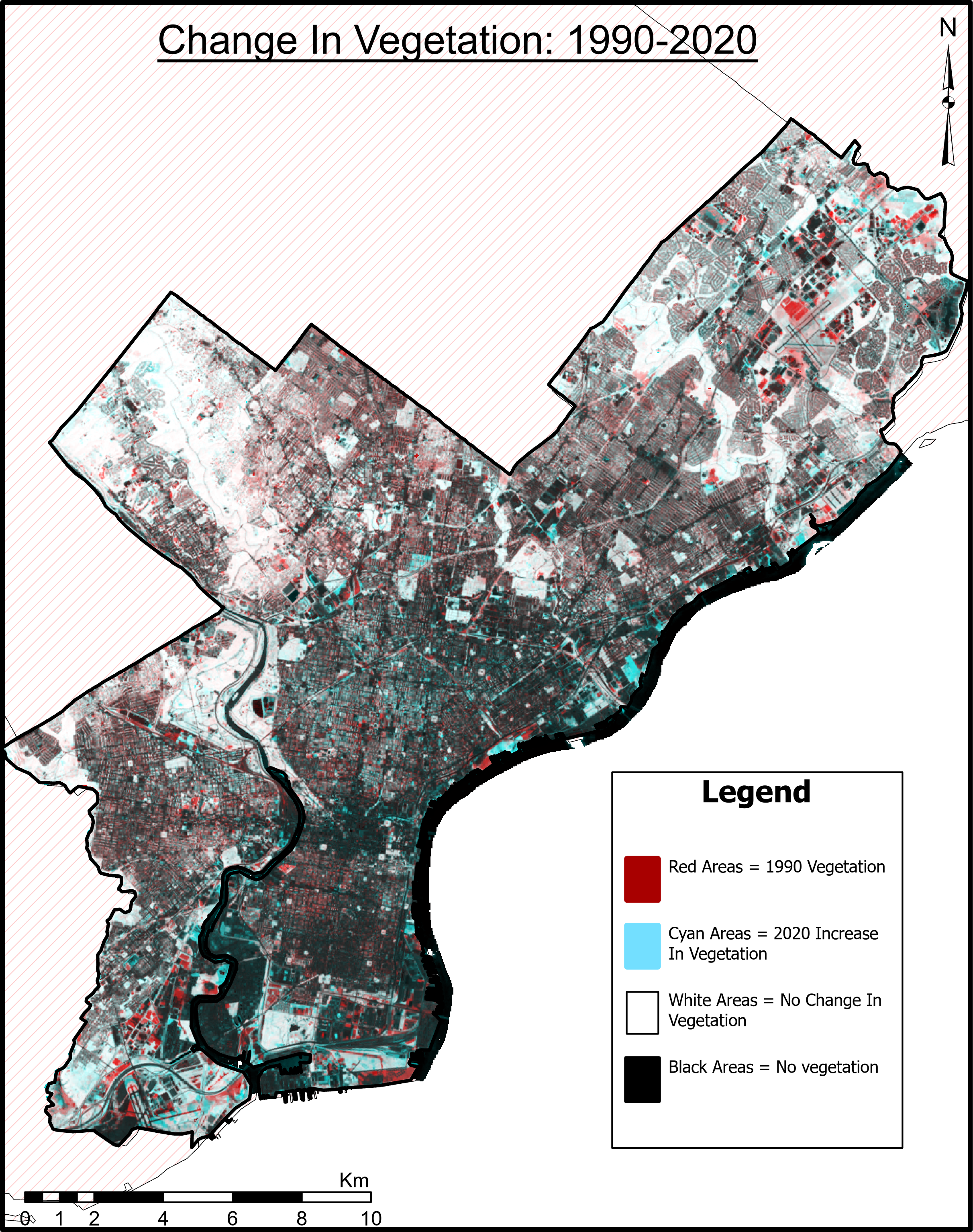
Greenness or green space is reflective of many different measures of quality of life, such as health disparities, racial residential segregation and urban heat islands, noise pollution, air quality, and lower income.
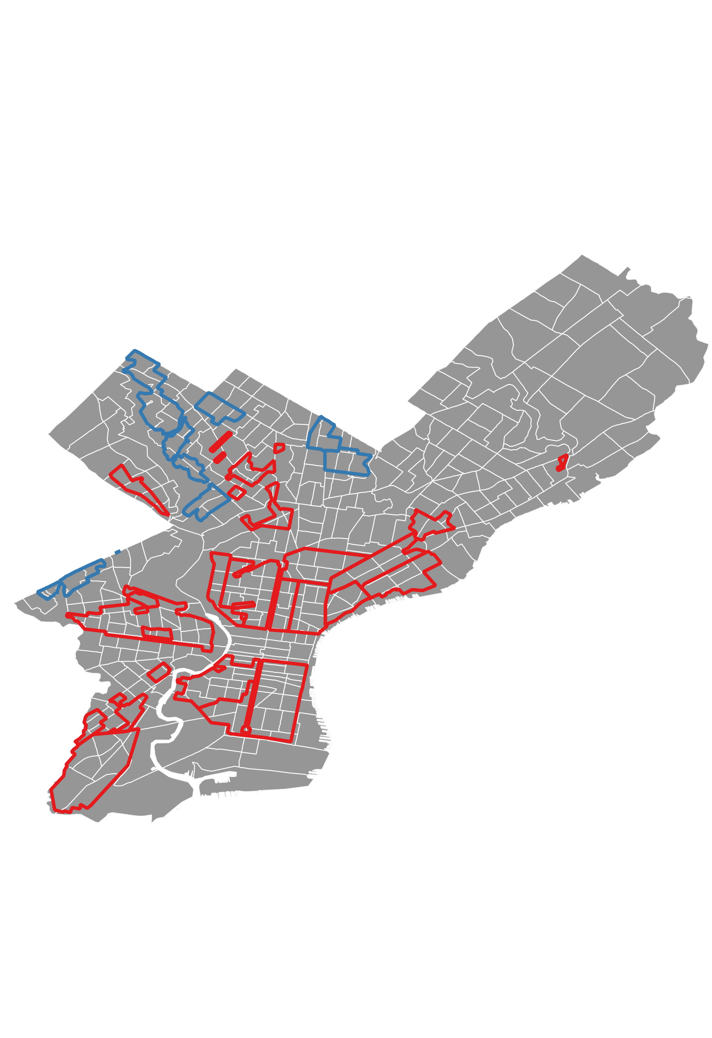
Using NDVI as a measure of greenness, the question is: How does NDVI change with income in the graded regions A and D of redlined maps in Philadelphia, PA?

- Calculate median NDVI for the years 1990, 2000, 2010, 2020 by U.S. census tract in each graded region.
- Median Income by tract from U.S. Census

- Explore data
- OLS to examine if there is statisically significant relationship of income & grading on NDVI
- Hypothesis testing comparing Mean NDVI based on grading and year.

Data Exploration
Two takeawys from this plot: 1. There are a significant amount of NDVI values with zero income, these are taken to be census tracts of open spaces. This interpretation does not mean address quality of the open space as they could be parks or abandoned lots.
- There outliers for both regions A and D.
The boxplots gives insight to the distribution of the two different regions for income and NDVI. The income median is always higher in regions graded A but region D has a greater shift towards higher values of income and outliers in 2020.
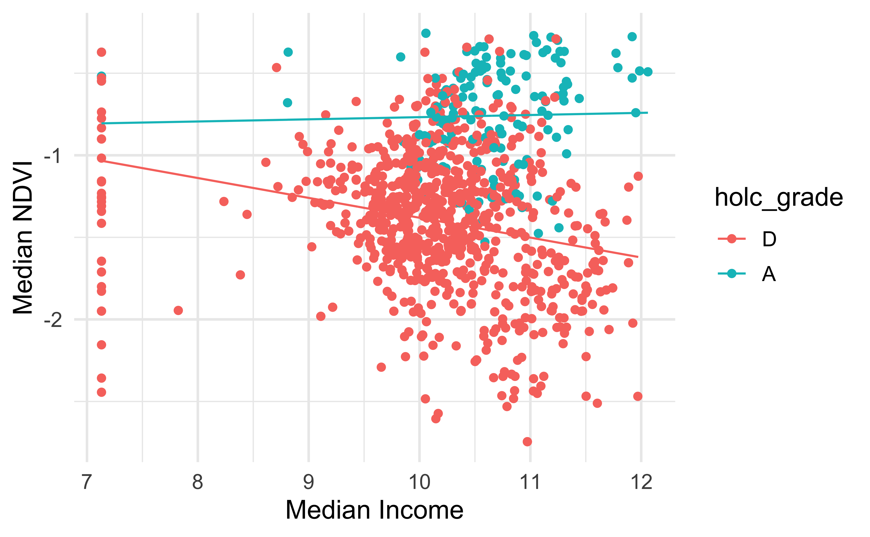
The first two distributions of income on the left and NDVI on the right indicate that a log-log transformation would be appropriate for the dataset. To perform a log-log transformation the zeros of income must be addressed. This being a spatial relationship simply removing did not seem appropriate, so the minimum value was found and divided in half replacing zeros in income.
The resulting log-log scatterplot after applying transformation and accounting for zeros.
Checking the OLS assumption that the X variable has variation.
var(ndvi_income0$income_mindiv2) != 0
#> [1] TRUE
Log-Log Ordinart Least Squares Regression
Our question is dependent on that we believe there is an interaction between income and grading resulting in different NDVI values. We first run the regression without the interaction to compare adjusted R-squared with the interaction.
\[ \text{log(NDVI)}_i = \beta_0 + \beta_1 \text{log(income)}_i \]
ADJUSTED R-SQUARED
mod <- lm(ndvi_log ~ income_log, data = ndvi_income0 )
summary(mod)$adj.r.squared
#> [1] 0.00791
#>
#> Call:
#> lm(formula = ndvi_log ~ income_log, data = ndvi_income0)
#>
#> Residuals:
#> Min 1Q Median 3Q Max
#> -1.3988 -0.2787 -0.0013 0.2654 1.1190
#>
#> Coefficients:
#> Estimate Std. Error t value Pr(>|t|)
#> (Intercept) -0.7662 0.1669 -4.59 4.9e-06 ***
#> income_log -0.0529 0.0163 -3.25 0.0012 **
#> ---
#> Signif. codes: 0 '***' 0.001 '**' 0.01 '*' 0.05 '.' 0.1 ' ' 1
#>
#> Residual standard error: 0.448 on 1198 degrees of freedom
#> Multiple R-squared: 0.00874, Adjusted R-squared: 0.00791
#> F-statistic: 10.6 on 1 and 1198 DF, p-value: 0.00119\[ \text{log(NDVI)}_i = \beta_0 + \beta_1 \text{log(income)}_i + \beta_2Grade + \beta_3log(income)*Grade + \varepsilon_i \]
A significant improved in Adjusted R-squared tells us adding the interaction of grade and income improves our model.
#> [1] 0.293summary(mod0)
#>
#> Call:
#> lm(formula = ndvi_log ~ income_log + holc_grade + income_log:holc_grade,
#> data = ndvi_income0)
#>
#> Residuals:
#> Min 1Q Median 3Q Max
#> -1.4104 -0.2260 0.0188 0.2382 1.2387
#>
#> Coefficients:
#> Estimate Std. Error t value Pr(>|t|)
#> (Intercept) -0.1703 0.1522 -1.12 0.2633
#> income_log -0.1210 0.0149 -8.12 1.2e-15 ***
#> holc_gradeA -0.7287 0.4422 -1.65 0.0996 .
#> income_log:holc_gradeA 0.1342 0.0420 3.19 0.0014 **
#> ---
#> Signif. codes: 0 '***' 0.001 '**' 0.01 '*' 0.05 '.' 0.1 ' ' 1
#>
#> Residual standard error: 0.378 on 1196 degrees of freedom
#> Multiple R-squared: 0.294, Adjusted R-squared: 0.293
#> F-statistic: 166 on 3 and 1196 DF, p-value: <2e-16Using 30 bins the residuals are mostly normally distributed over zero with a slight left tail.
As a whole there is some consistency in the distribution of the variance but when looked at as two distinct groups as picured here the distribution is much greater. This threathens assumption 4 of OLS,
Interpretation of Coefficients
\[ \small {log(NDVI)}_i = -0.170 + (-0.121){log(income)}_i + (-0.729)Grade + (0.134)log(income)*Grade + \varepsilon_i \small \]
| term | estimate | std.error | statistic | p.value |
|---|---|---|---|---|
| (Intercept) | -0.170 | 0.1522 | -1.12 | 2.63e-01 |
| income_log | -0.121 | 0.0149 | -8.12 | 1.18e-15 |
| holc_gradeA | -0.729 | 0.4422 | -1.65 | 9.96e-02 |
| income_log:holc_gradeA | 0.134 | 0.0420 | 3.19 | 1.44e-03 |
Intercept: the coefficient is -0.170. For every 1% increase in the independent variable income, our dependent variable NDVI decreases by 0.17%.
For every 1% increase in the independent variable INCOME, our dependent variable NDVI DECREASES by about 32.59” For region graded D, our dependent variable NDVI DECREASES by about 17.75
The percentage of the impact of region grade on NDVI, is 42.07 higher in Region graded A than it is in region graded D.

Hypothesis Testing
- \[H_{0}: \mu_{ndvi20gradeD} - \mu_{ndvi90gradeD} = 0 \] \[H_{A}: \mu_{ndvi20gradeD} - \mu_{ndvi90gradeD} \neq 0\]
#>
#>  Welch Two Sample t-test
#>
#> data:  ndvi_income_20$ndvi[ndvi_income_20$holc_grade == "D"] and ndvi_income_90$ndvi[ndvi_income_90$holc_grade == "D"]
#> t = -12, df = 455, p-value <2e-16
#> alternative hypothesis: true difference in means is not equal to 0
#> 95 percent confidence interval:
#>  -0.118 -0.084
#> sample estimates:
#> mean of x mean of y
#>     0.213     0.315
\[H_{0}: \mu_{Income20gradeD} - \mu_{Income90gradeD} = 0 \] \[H_{A}: \mu_{Income20gradeD} - \mu_{Income90gradeD} \neq 0\]
#>
#>  Welch Two Sample t-test
#>
#> data:  ndvi_income_20$income[ndvi_income_20$holc_grade == "D"] and ndvi_income_90$income[ndvi_income_90$holc_grade == "D"]
#> t = 15, df = 322, p-value <2e-16
#> alternative hypothesis: true difference in means is not equal to 0
#> 95 percent confidence interval:
#>  25408 33297
#> sample estimates:
#> mean of x mean of y
#>     49443     20091
We reject the null hypothesis that the differnce in means is equal to zero. The hypothesis test p-value is very small, so our results are significant in that there is a difference in means.
In examining the results we see that the values of the means we can see that there is a decrease in NDVI when comparing 2020 to 1990. This leads to the second hypothesis test of comparing the means in income.
The p-value again informs that our results are statistically significant and that we reject the null hypothesis.
This relationship is not what we expected in that income increased from 1990 to 2020, but NDVI decreased.
Region A VS D in 2020
Finally to answer our initial question we compare two different graded regions in both their difference in NDVI and income.
\[H_{0}: \mu_{ndvi20gradeA} - \mu_{ndvi20gradeD} = 0 \]
\[H_{A}: \mu_{ndvi20gradeA} - \mu_{ndvi20gradeD} \neq 0\]
#>
#>  Welch Two Sample t-test
#>
#> data:  ndvi_income_20$ndvi[ndvi_income_20$holc_grade == "A"] and ndvi_income_20$ndvi[ndvi_income_20$holc_grade == "D"]
#> t = 9, df = 48, p-value = 3e-12
#> alternative hypothesis: true difference in means is not equal to 0
#> 95 percent confidence interval:
#>  0.135 0.209
#> sample estimates:
#> mean of x mean of y
#>     0.385     0.213
#>
#> Welch Two Sample t-test
#>
#> data: ndvi_income_20$income[ndvi_income_20$holc_grade == "A"] and ndvi_income_20$income[ndvi_income_20$holc_grade == "D"]
#> t = 0.1, df = 60, p-value = 0.9
#> alternative hypothesis: true difference in means is not equal to 0
#> 95 percent confidence interval:
#> -8533 9559
#> sample estimates:
#> mean of x mean of y
#> 49957 49443When it comes to NDVI the results are statistically significant as the p-value is very small. The mean is higher in a region graded A compared to a region graded D.
With regard to income and a p-value of 0.9 we fail to reject the null hypothesis that there that the true difference of means is equal to zero at \(\alpha =0.5\)
I read this as that even though incomes have risen in regions in graded D to be statistically indiscernible from regions graded A, there is a statistically significant difference in greenness in the two regions and the greeness has decreased in D regions.
Conclusion
The interpretations of the final hypothesis test tell us that there is a difference in regions graded A versus D but that they do not follow with income. The p-value of 0.09 in the linear regression for grade suggest that grade alone is not a significant indicator of NDVI but the interaction with income and its very low p-value that it should be considered. Further exploration of the relationship between incoming and grading and NDVI should include more of the spatial component and conitnous data if possible.
Data and Code
The data used for this project can be found here:
NDVI and Income by Census Tract
The code for processing this file is within this post source file:
OR the scratch repository used to create the in-class presentation:
References
The log-0 problem: analysis strategies and options for choosing c in log(y + c) (rbind.io)
Nardone, Anthony, et al. “Redlines and Greenspace: The Relationship between Historical Redlining and 2010 Greenspace across the United States.” National Institute of Environmental Health Sciences, U.S. Department of Health and Human Services, 27 Jan.2021, https://ehp.niehs.nih.gov/doi/10.1289/EHP7495.
Casey, J.A.; James, P.; Cushing, L.; Jesdale, B.M.; Morello-Frosch, R. Race, Ethnicity, Income Concentration and 10-Year Change in Urban Greenness in the United States. Int. J. Environ. Res. Public Health 2017, 14, 1546, doi.org/10.3390/ijerph14121546
https://romero61.github.io/posts/redlining_NDVI.html
Schwarz, K., Fragkias, M., Boone, C.G., Zhou, W., McHale, M., Grove, J.M., O’Neil-Dunne, J., McFadden, J.P., Buckley, G.L., Childers, D., Ogden, L., Pincetl, S., Pataki, D., Whitmer, A. and Cadenasso, M.L. (2015). Trees Grow on Money: Urban Tree Canopy Cover and Environmental Justice. PLOS ONE, [online] 10(4), p.e0122051. doi:10.1371/journal.pone.0122051.
